Today I’d like to teach you how to solve a pole placement problem. The table of contents is shown below.
[Example Problem]
Consider the system given by
$$\dot{\boldsymbol{x}}(t)=
\begin{bmatrix}
-4 & 0 & 6\\
1 & 0 & -3\\
0 & 1 & -2
\end{bmatrix}\boldsymbol{x}(t)
+
\begin{bmatrix}
1\\
0\\
0
\end{bmatrix}u(t)$$
and then derive feedback gains that place poles of a closed-loop system at -4, -5, and -6.
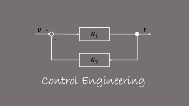
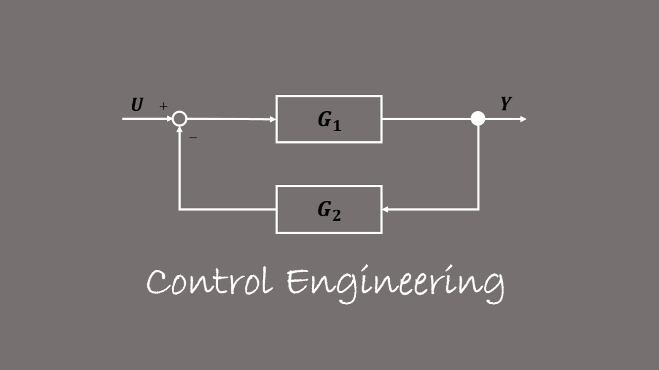
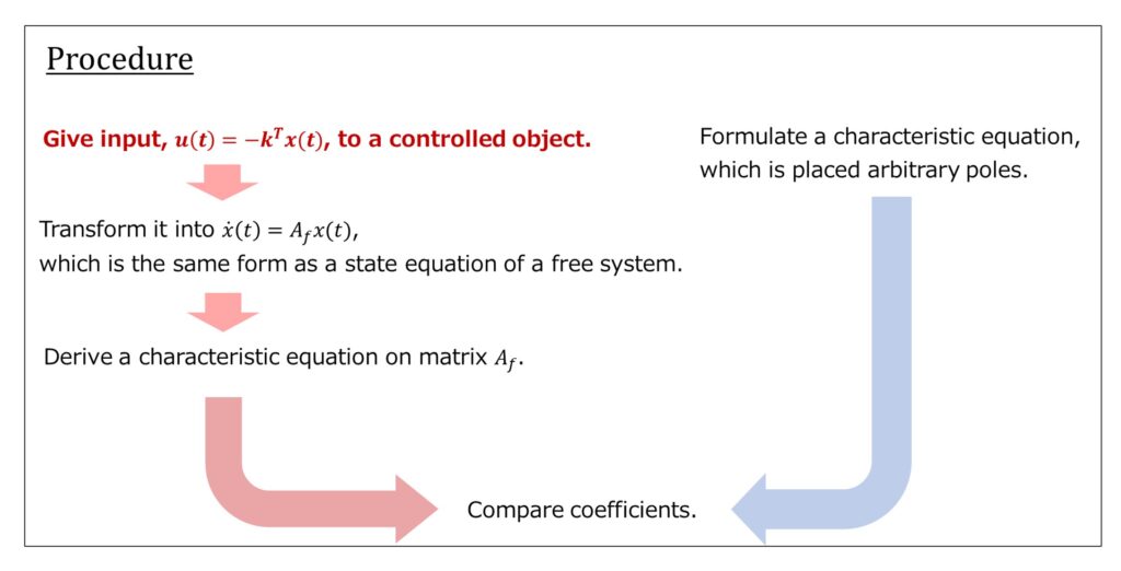
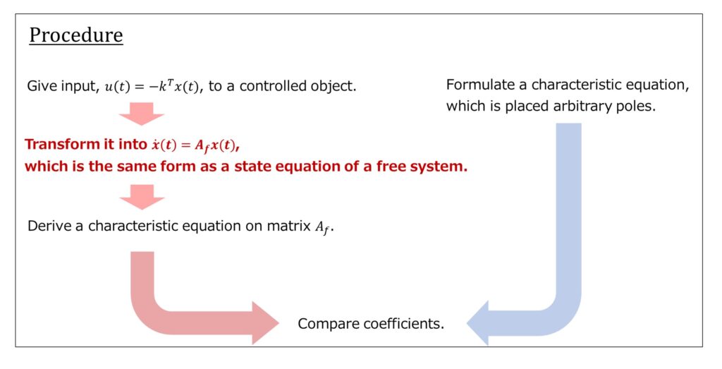
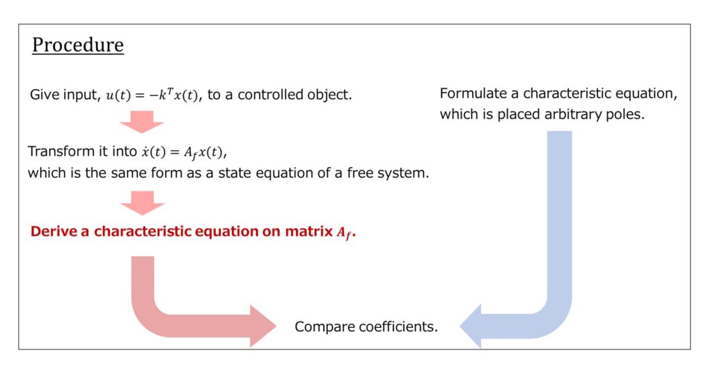
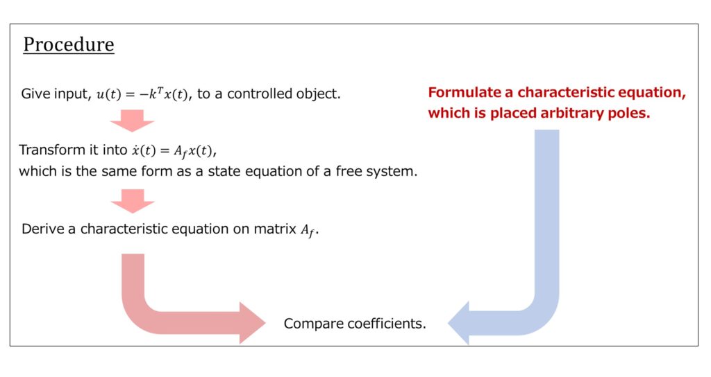
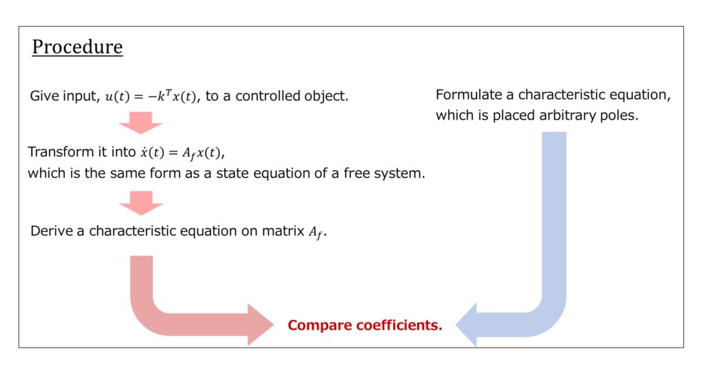
Give input, \(𝑢(𝑡)=−\boldsymbol{𝑘}^{T} \boldsymbol{𝑥}(𝑡)\), to a controlled object.
You can transform it into the following state feedback system with control law, \(u(t)=-\boldsymbol{k}^T \boldsymbol{x}(t)\).
\begin{eqnarray}
\dot{x}(t) &=& A \boldsymbol{x}(t)+\boldsymbol{b}u(t)\\
&=& A\boldsymbol{x}(t) +\boldsymbol{b}(-\boldsymbol{k}^{T} \boldsymbol{x}(t))
\end{eqnarray}
Transform it into \(\dot{\boldsymbol{x}}(t)=A_{f}\boldsymbol{x}(t)\), which is the same form as a state equation of a free system.
\begin{eqnarray}
\dot{\boldsymbol{x}} &=& A\boldsymbol{x}(t) + \boldsymbol{b}(-\boldsymbol{k}^{T} \boldsymbol{x}(t))\\
&=& (A – \boldsymbol{bk^{T}}) \boldsymbol{x}(t)\\
&=& A_{f}\boldsymbol{x}(t)
\end{eqnarray}
However, matrix \(A_{f}\) is shown as follows.
\begin{eqnarray}
A_{f} &=& A-\boldsymbol{bk}^{T}\\
&=&
\begin{bmatrix}
-4 & 0 & 6\\
1 & 0 & -3\\
0 & 1 & -2
\end{bmatrix}-
\begin{bmatrix}
1\\
0\\
0
\end{bmatrix}
\begin{bmatrix}
k_{1} & k_{2} & k_{3}
\end{bmatrix}\\
&=&
\begin{bmatrix}
-4 & 0 & 6\\
1 & 0 & -3\\
0 & 1 & -2
\end{bmatrix}-
\begin{bmatrix}
k_{1} & k_{2} & k_{3}\\
0 & 0 & 0\\
0 & 0 & 0
\end{bmatrix}\\
&=&
\begin{bmatrix}
-4-k_{1} & -k_{2} & 6-k_{3}\\
1 & 0 & -3\\
0 & 1 & -2\\
\end{bmatrix}
\end{eqnarray}
Derive a characteristic equation on matrix \(A_{f}\)
Find a characteristic polynomial of the closed-loop system.
\begin{eqnarray}
s\boldsymbol{I}-A_{f} &=&
\begin{bmatrix}
s & 0 & 0\\
0 & s & 0\\
0 & 0 & s\\
\end{bmatrix}-
\begin{bmatrix}
-4-k_{1} & -k_{2} & 6-k_{3}\\
1 & 0 & -3\\
0 & 1 & -2\\
\end{bmatrix}\\
&=&
\begin{bmatrix}
s+4+k_{1} & k_{2} & -6+k_{3}\\
-1 & s & 3\\
0 & -1 & s+2\\
\end{bmatrix}
\end{eqnarray}
When the cofactor expansion is performed in the first column, you can find a characteristic polynomial as follows.
\begin{eqnarray}
det(s\boldsymbol{I} – A_{f}) &=& (-1)^{1+1} \cdot (s+4+k_{1}) \cdot
\begin{vmatrix}
s & 3\\
-1 & s+2\\
\end{vmatrix} + (-1)^{2+1} \cdot (-1) \cdot
\begin{vmatrix}
k_{2} & -6+k_{3}\\
-1 & s+2\\
\end{vmatrix}\\
&=&
s^{3}+(6+k_{1})s^{2}+(11+2k_{1}+k_{2})s+(6+3k_{1}+2k_{2}+k_{3})
\end{eqnarray}
Formulate a characteristic equation, which is placed arbitrary poles.
Also, a characteristic polynomial that has poles at -4, -5, and -6 is given by the following formula.
$$(s+4)(s+5)(s+6)=s^{3}+15s^{2}+74s+120$$
Compare coefficients.
Compare coefficients.
\begin{cases}
6+k_{1}=15\\
11+2k_{1}+k_{2}=64\\
6+3k_{1}+2k_{2}+k_{3}=120\\
\end{cases}
Also, solving the system of equations, you get the following feedback gains.
\begin{cases}
k_{1}=9\\
k_{2}=45\\
k_{3}=-3
\end{cases}